

Word to the reader: That is the fourth in a collection of articles I am publishing right here taken from my e book, “Investing with the Pattern.” Hopefully, one can find this content material helpful. Market myths are typically perpetuated by repetition, deceptive symbolic connections, and the entire ignorance of details. The world of finance is stuffed with such tendencies, and right here, you will see some examples. Please remember the fact that not all of those examples are completely deceptive — they’re generally legitimate — however have too many holes in them to be worthwhile as funding ideas. And never all are instantly associated to investing and finance. Get pleasure from! – Greg
As an aerospace engineer, my training stored me far faraway from the world of finance. Nonetheless, over the previous couple of many years, my profession has since dropped me solidly into that world.
The “world of finance” is my baked-up time period that features monetary academia and, on the whole, retail (promote facet) Wall Road. (I actually imagine that the previous is the advertising and marketing division of the latter.)
In engineering, we knew that with the intention to start an evaluation or delve right into a analysis undertaking, we needed to begin with some fundamental assumptions about issues. These assumptions have been the constructing blocks for the undertaking; they launch the method. Many occasions, effectively into the undertaking, it could be apparent that a few of the assumptions have been simply incorrect and needed to be corrected or eliminated. The World of Finance, over the previous 60 years, has produced numerous white papers on monetary theories, a lot of which start with some fundamental assumptions.
- The markets are environment friendly.
- Traders are rational.
- Returns are random.
- Returns are usually distributed.
- Gaussian (bell-curve) statistics is suitable to be used in finance/investing.
- Alpha and beta are impartial of correlation.
- Volatility is danger.
- Is a 60 p.c fairness/40 p.c fastened earnings acceptable?
- Evaluate ahead (guesses) Worth Earnings (PE) with long-term trailing (reported) PE.
The rest of this part covers the challenges I’ve for the above checklist. Personally, I believe fashionable finance is nearly a hoax, an space of investments that has proliferated into a big gross sales pitch. Few problem it, and even fewer absolutely perceive it. I believe I might write a complete e book in regards to the flaws of contemporary finance, however will attempt to provide quite a few examples of how shallow and really ineffective a few of the ideas are, together with examples. Hopefully, I shall be profitable sufficient with a few of these that it’s going to no less than convey concern in your half and entice additional examine into the topic.
I ought to state that this is not a lot in regards to the issues of contemporary finance as it’s with how funding administration cherry-picks and misuses components of it for advertising and marketing functions.
What Trendy Portfolio Idea Forgot or Ignored
Recall that the idea assumes that every one buyers acquire the identical data on the identical time, and likewise that they react equally and share the identical funding objectives. Listed below are some rhetorical inquiries to problem these assumptions:
Do individuals commerce/make investments utilizing completely different time horizons? There at the moment are buyers/ merchants who commerce in extraordinarily brief intervals through the day. There are those that won’t ever maintain a place in a single day. There are those that let the market decide their holding interval. And there are those that purchase and maintain for very lengthy intervals of time.
Are there completely different views of danger amongst buyers? The actually unhappy a part of this query is that the majority buyers don’t absolutely perceive danger and positively have no idea what their danger tolerance is, not to mention apply it to an funding technique.
Are there completely different views of the place the identical inventory’s value shall be one week, one month, or one yr from now? This does not want any rationalization, as a result of for those who learn monetary media or watch tv, you already know there may be an infinite provide of opinions on this.
The Capital Asset Pricing Mannequin (CAPM) assumes that buyers agree on return, danger, and correlation traits of all property and make investments accordingly. They not often do. Among the issues with return, danger, and correlations are handled elsewhere on this e book. The most important is that the majority use very long-term averages of those to evaluate future valuations. They need to use a median that adapts to an investor’s investing time horizon.
Trendy Portfolio Idea and the Bell Curve
I am going to let Benoit Mandelbrot clarify it from his e book, The (Mis)Habits of Markets (p. 13). The bell curve suits actuality fairly poorly. From 1916 to 2003, the day by day actions of the Dow Industrials don’t unfold out on graph paper like a easy bell curve. The far edges flare too excessive. Idea means that over that point, there must be 58 days when the Industrials moved greater than 3.4 p.c; actually, there are 1,001 such days. Idea predicts six days of swings past 4.5 p.c; actually, there have been 366. And swings of greater than 7 p.c ought to come as soon as each 300,000 years; actually, there have been 48 such days. Maybe the assumptions have been incorrect.
Black Monday, October 19, 1987
“The Dow Jones Industrials fell 29.2 p.c. The chance of that occuring, primarily based on the usual reckoning of monetary theorists, was one in 10 to the fiftieth energy; odds so small that they haven’t any that means. It’s a quantity exterior the dimensions of nature. You possibly can span the powers of ten from the smallest subatomic particle to the breadth of the measurable universe—and nonetheless by no means meet such a quantity.” — The (Mis)Habits of Markets, Benoit Mandelbrot.
With out realizing how he calculated the returns (day by day, weekly, and so forth.) and the quantity of knowledge used within the calculation, it’s unimaginable to re-create his numbers. He said that on Black Monday the Dow Industrials fell 29.2 p.c. Listed below are the numbers: October 16, 1987, shut value was 2,246.74; October 19, 1987, shut value was 1,738.74, a decline of twenty-two.61%. If one used the low of October 19, 1987 (1,677.55), the decline can be 25.33%. The message, nonetheless, is identical; it was an enormous decline and one which statistically ought to by no means occur.
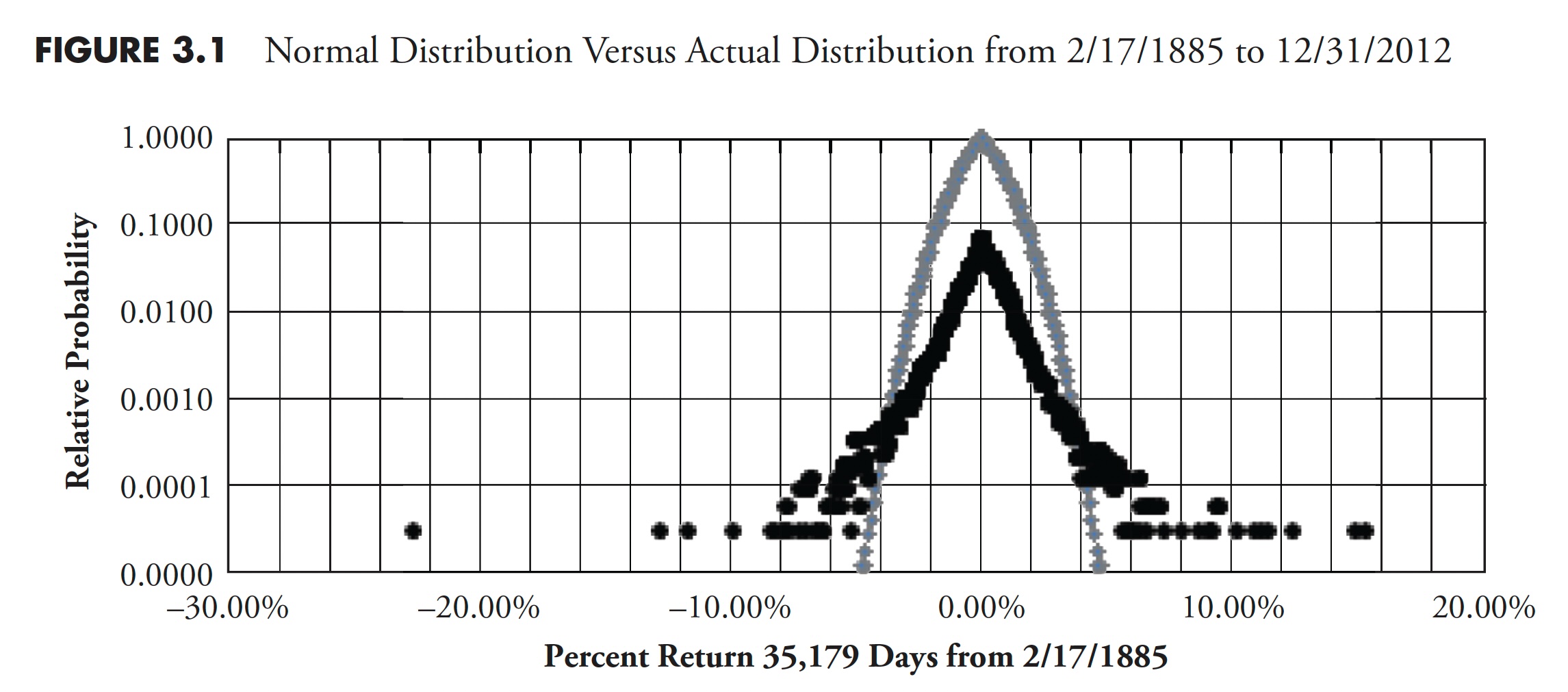 Determine 3.1
Determine 3.1 exhibits the large distinction between the distribution of returns from the Gaussian “regular distribution” and the precise distribution of empirical information. That is the day by day return of the Dow Industrials from 1885 with the vertical axis being relative chance and the horizontal axis being p.c return. The taller peak is the Gaussian regular distribution and the opposite is the precise returns. You possibly can see the small dot on the far left representing the .22.61 p.c day often called Black Monday, October 19, 1987.
Tails Wagging the Canine
If an asset bubble is outlined as 2 normal deviations (σ, sigma) about its imply, then… statistically it will not occur however as soon as each 43 years (4 sigma whole). Statistics dictate that solely as soon as each 1,600 years ought to such occasions be adopted by a reverse transfer downward of two normal deviations. Sadly, these occasions occur typically. Therefore, as soon as once more, Gaussian statistics will not be acceptable for market information.
October 2008 had some uncommon occasions. Desk 3.1 exhibits 11 days throughout October 2008, ordered by absolute day by day return.
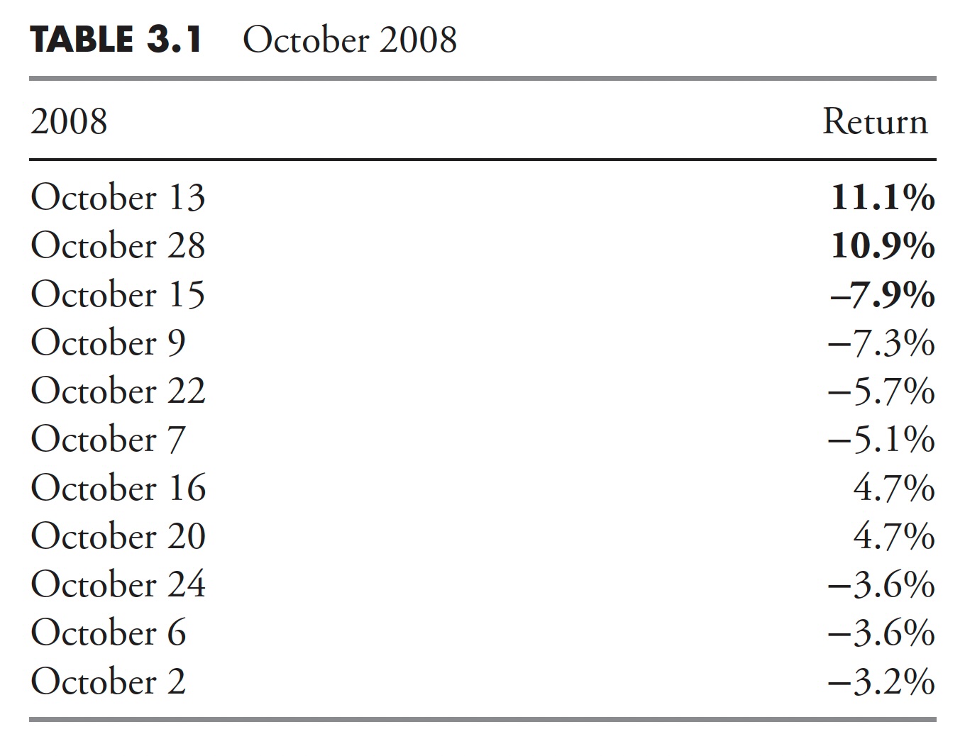 Desk 3.1
The highest three days primarily based upon absolute day by day returns are 11.1 p.c, 10.9 per.cent, and .7.9 p.c. The mathematical odds of three days with larger than 7.9 p.c strikes is 1 in 10,000,000,000,000,000,000,000 (that is 10 plus 21 zeros). The rise of the time period “fats tails” occurred as a result of the world of finance makes use of the incorrect statistical evaluation for the market. If the right evaluation have been used, the time period fats tails wouldn’t be used, it could have been addressed. This instance jogs my memory of the e-Commerce child exclaiming that the percentages are the identical as being eaten by a polar bear and a daily bear in the identical day. Whereas I ‘m essential of the statistics utilized in fashionable finance, I believe I ‘m extra involved about their widely-held perception as being legitimate. If you already know one thing has issues, you’ll be able to alter accordingly. If you don’t understand there are issues, you’re in hassle.
My pal Ted Wong (TTSWong Advisory) has this to say about fashionable finance: “After Markowitz launched Trendy Portfolio Idea (MPT) within the Nineteen Fifties, which was primarily based on the Gaussian speculation, most theoreticians had since moved away from Gaussian statistics. Solely the naive analysis analysts within the monetary wire-houses and mutual fund establishments nonetheless use regular distributions of their papers. In truth, Benoit Mandelbrot, cited in your e book, was the primary to level out, within the mid-Nineteen Sixties, that the bell curve couldn’t clarify many fats tails noticed in nature and within the monetary markets. Fama and French identified that Gaussian statistics was solely a particular case within the household of Paretian distributions. The latter might account for all types of fats tails by adjusting the leptokurtosis coefficient.”
Creator’s observe: Paretian refers to steady distributions, which must be utilized in fashionable finance however not often are as a result of the arithmetic is extra advanced; anyway, that’s my opinion. James Weatherall, in The Physics of Wall Road, supplies a singular historical past of how Mandelbrot challenged fashionable finance and made headway, however in the end didn’t change something.
“To me, the underlying downside with fashionable finance shouldn’t be that Gaussian distributions do not match the fats tails effectively. By adjusting the leptokurtosis coefficient, the quasi-bell curve can now be bent by the theoreticians to no matter shapes and types to suit the empirical information. The actual problem in fashionable finance is the “blind” religion within the random stroll speculation. Each the MPT and the Paretian practitioners assume that market costs behave in a random vogue. The random stroll doctrine assumes that value adjustments are impartial variables; that’s, at present’s value change has no relationship with yesterday’s or tomorrow’s value change. They’ve a whole lot of “proofs” to again up that declare and in consequence, monetary academia laughs at technical and even elementary analysts of their efforts to foretell future market costs.
“What the random walkers miss is the truth that most technical and quantitative analyses will not be supposed for predicting day by day value adjustments, which I agree are kind of random. We imagine that market costs will not be random over an extended time period. The distributions of completely random value occasions ought to have the imply close to 0% and surrounded by a symmetrical distribution on both facet, similar to the bell curve or the Paretian curve (with fats tails on each side). If the imply return is situated off heart and the distributions are asymmetrical across the imply, then one can absolutely problem the notion of randomness. Nicely, have a look at your Determine 2.1; it is a clear demonstration that over a one-year interval, the imply p.c return is off-center to the best, and the distributions are asymmetrical across the imply. Therefore the historic annual return histogram proves that the market shouldn’t be random. The longer the holding interval, the much less random (thus extra predictable) the market is! Random walks are solely random when one walks a short while distance. One can rightfully say that day merchants are true random walkers and that technical evaluation is probably not as helpful to them.”
Commonplace Deviation (Sigma) and Its Shortcomings
(Warning: This part is for nerds solely!)
Definition: A light-weight yr is a distance, not a time. It’s the distance that mild will journey in a single yr.
Desk 3.2 has some numbers which might be past human capability to think about. They’re past our potential to grasp. In my regular overkill vogue, my aim right here is to place these large numbers right into a plausible perspective so you’ll imagine that one thing is incorrect with the statistics of contemporary finance. Black Monday, October 19, 1987, was a decline of twenty-two.61 p.c, which was roughly 22 sigma. Twenty-two sigma as proven in Desk 3.2, primarily based on Gaussian statistics, ought to solely happen as soon as in each 9.5 x 10^103 years. That must be put into perspective. The velocity of sunshine is roughly 186,282 miles per second, so the velocity of sunshine in miles per hours is 186,282 x 60 x 60 = 670,615,200 miles per hour. Additional growth exhibits that the velocity of sunshine per day is 670,615,200 x 24 = 16,094,764,800 miles per day, and so the velocity of sunshine per yr is 16,094,764,800 x 365.25 = 5,878,612,843,200 miles per yr. In scientific notation that is expressed as 5.878 x 10^12. Word that this quantity is much like the worth for eight sigma (see Desk 3.2 ). To create an impression of sigma that’s larger than eight would require using phrases that cope with the universe, but I will give it a shot.
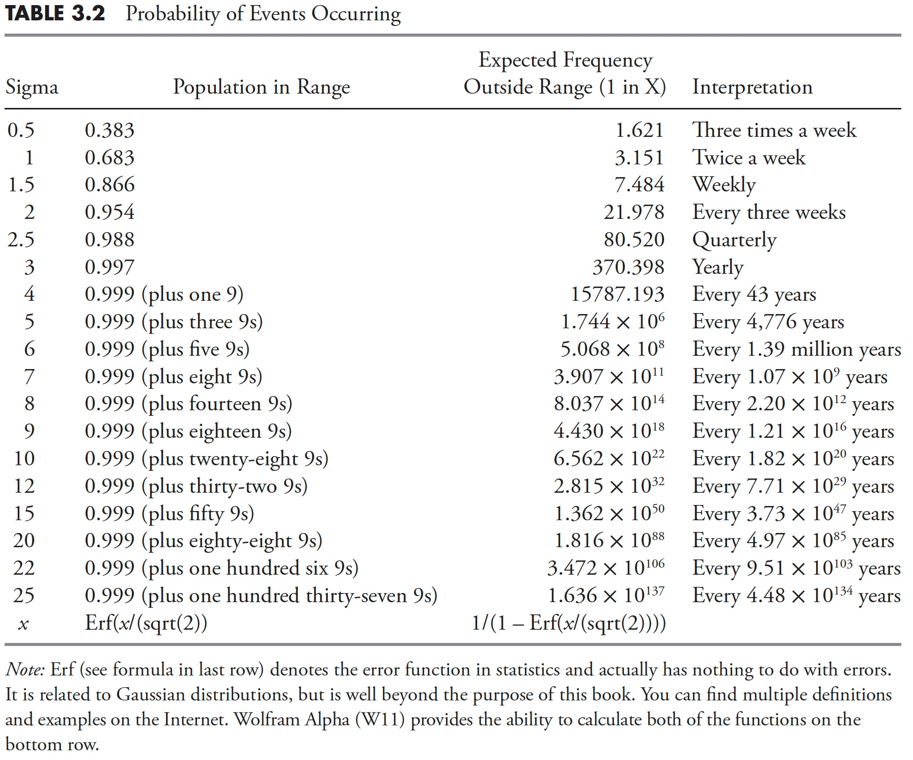 Desk 3.2
Here’s a checklist of galactic-like measurements to assist put large-sigma occasions into perspective. There are various fantastic web sites on astronomy and such. I checked quite a few them and located a basic settlement with the numbers utilized in these examples. Remember the fact that the numbers have been generated with a scientific strategy, not only a guess, however nonetheless could possibly be in appreciable error. A lot of the data might be discovered on www.universetoday.com.
What number of stars are there within the Milky Method galaxy? I discovered that, many alternative sources, this quantity was pretty constant — about 2,500 seen to the bare eye on Earth at anybody time, and 5,800 to eight,000 whole seen stars. Now right here is the guess of astronomers for the entire variety of stars within the Milky Method: 200 billion to 400 billion (4 x 10^12). Now the Milky Method galaxy is a spiral galaxy that’s roughly 100,000 mild years throughout, so you’ll be able to see that we really have no idea a exact reply apart from there are billions of stars within the Milky Method galaxy.
What number of galaxies are within the universe? As a result of we are able to solely see a fraction of the universe, that is unimaginable to know, however most astronomers have mentioned that there are 100 billion to 200 billion galaxies within the universe. Their current supercomputer put the quantity at greater than 500 billion; in different phrases, there may be a complete galaxy for each star within the Milky Method.
The plain subsequent query, then, is what number of stars within the universe? Because the dedication for the variety of galaxies within the universe and the variety of stars in every galaxy is clearly a wide-ranging estimate, I am going to simply use one thing close to the center of the estimates (aren’t you glad I did not use common?). Then, 400 billion galaxies and 400 billion stars in every galaxy equate to 160 trillion stars within the universe. In scientific notation, that’s (4 x 10^12) x (4 x 10^12) = 1.6 x 10^25 . That is lots of stars, however remember the fact that the aim of this cosmic train is to get a perspective on excessive sigma occasions. Desk 3.2, you’ll be able to see that that is near about an 11-sigma occasion.
What number of atoms within the universe? Let’s use the extra conservative of the estimates, simply to maintain it thrilling. If there are 300 billion galaxies within the universe, and the variety of stars in a galaxy might be 400 billion, then the entire variety of stars within the universe can be about 1.2 x 10^23. At all times consult with the sigma desk to see the place these numbers stand relative to large-sigma occasions to maintain them in perspective. UniverseToday estimates that, on common (there’s that idea once more), every star can weigh 10^35 grams. Subsequently, the entire mass of the universe can be about 10^58 grams (Word: Multiplication of exponents is simple, simply add them: 23 + 35 = 58). As a result of a gram of matter is understood to have about 10^24 protons (identical because the variety of hydrogen atoms), then the entire variety of atoms within the universe is about 10^82 . From Desk 3.2, you’ll be able to extrapolate and see that it’s about the identical as a 19-sigma occasion occurring—and Black Monday, October 19, 1987, was a 22-sigma occasion.
What’s the age of the universe? NASA’s Wilkinson Microwave Anisotropy Probe has pegged the reply to 13.73 billion years, with a margin of error all the way down to solely 120 million years (1.2 x 10^8).
What’s the age of the Earth? Plate tectonics has triggered rocks to be recycled, which makes it tough to truly decide the Earth’s age. They’ve discovered rocks in Michigan and Minnesota which might be about 3.6 billion years outdated (3.6 x 10^9). Western Australia has yielded the oldest rocks so far at 4.3 billion years. Moon rocks and meteorites have yielded about 4.54 billion years on common, which can be science’s dedication for the age of the photo voltaic system.
What about people? Presently (appears they’re at all times discovering one thing older) the primary Homo habilis developed about 2.3 million years in the past—these have been the parents that used stone instruments and regarded most likely not too completely different than a chimp. In line with Current African Ancestry principle, fashionable people developed in Africa and migrated out of the continent about 50,000 to 100,000 years in the past. The forerunner for anatomically fashionable people developed between 400,000 and 250,000 years in the past. Lastly, many anthropologists agree that the transition to behavioral modernity (tradition, language, and so forth.) occurred about 50,000 years in the past. We people are actually a tiny fraction in comparison with the universe, and, specifically, massive sigma occasions.
Okay, I’ve totally beat this “perspective” concept to loss of life however hope you discovered the galactic data entertaining. Mainly, and virtually, any sigma larger than 4 is normally addressed as infinity. Furthermore, within the case of the inventory market, meaning these occasions ought to by no means occur, but they do. And method too typically!
Desk 3.2 exhibits numerous sigma, the p.c of inhabitants, the chance of exceeding that sigma, and a calendar-based interpretation. I’ve seen that Microsoft Excel and Wolfram Alpha produce barely completely different values. I believe that, even with one of the best of intentions when coping with extraordinarily massive or small numbers, one easy rounding error or inappropriate rounding can result in variations; nonetheless, it didn’t have an effect on the message right here.
Improper Course of
When diving into this undertaking on normal deviation and huge market strikes, I spotted that, all too typically, analysts who’re exhibiting related data are making an egregious error within the calculation. In case you needed to know the usual deviation (sigma) for October 19, 1987 (Black Monday), then you definately can not use any information later than or together with that day to find out it. I see many occasions that one will use the calculation of ordinary deviation every day as much as the day of the evaluation, which regularly contains a few years of knowledge that didn’t exist on the time of the occasion being analyzed. Desk 3.3 exhibits the ten largest share days within the Dow Industrials since 1885. The Right Sigma column exhibits the calculation for previous information as much as the day earlier than the occasion, whereas the Spot Sigma column exhibits the calculation for the day in query utilizing all the information obtainable as much as 12/31/2012, which I do not imagine is legitimate. Nonetheless, you’ll discover that there’s not an enormous distinction within the two columns; that’s, till you have a look at the distinction and put it right into a perspective that the human mind can cope with.
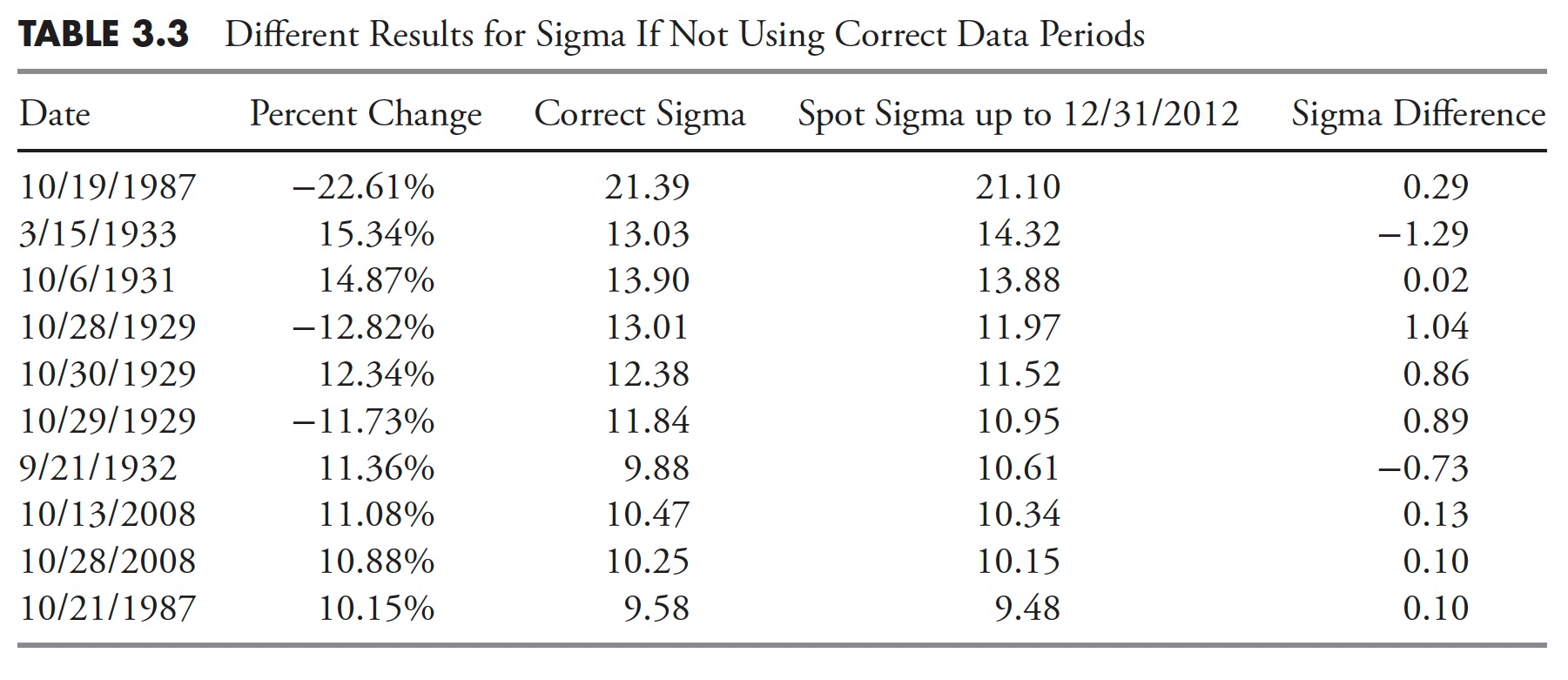 Desk 3.3
Excessive Sigma Days We All Bear in mind
In an try and painting sure days previously that we have now heard a lot about, the calculation of sigma anticipated and noticed previous to these days is offered right here for occasions from one sigma as much as and together with eight sigma. You’ll discover that on the excessive sigma information within the tables a few of the information was completely too massive or too small to incorporate. Additionally, the times we’re discussing within the part have been all a lot larger than 8-sigma days. This evaluation is to as soon as once more present how typically we expertise strikes available in the market that our fully past the boundaries of contemporary finance. Listed below are the reasons of the headers within the following three tables, October 28 to 29, 1929, October 19, 1987, and all the information as much as 12/31/2012.
Sigma—Commonplace deviation.
AM – xSD—P.c transfer representing the typical imply (AM) much less an “x” sigma transfer.
Anticipated—The variety of occasions anticipated utilizing statistics.
Noticed—The precise variety of occasions.
Ratio—The ratio of anticipated to noticed occasions.
AM + xSD—P.c transfer representing the typical imply (AM) plus an “x” sigma transfer.
Anticipated—The variety of occasions anticipated utilizing statistics.
Noticed—The precise variety of occasions.
Ratio—The ratio of anticipated to noticed occasions.
Complete Anticipated—The full of occasions anticipated above and under the imply.
Complete Noticed—The full of precise occasions above and under the imply.
Ratio—The ratio of the Complete Anticipated and Complete Noticed occasions.
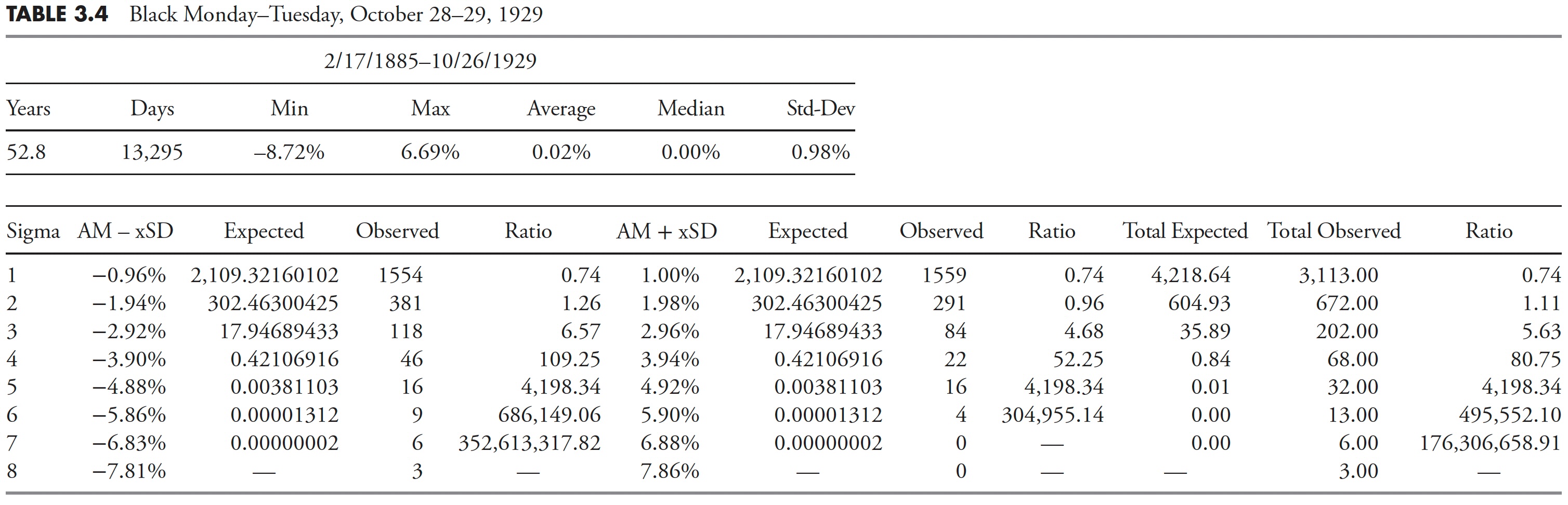
Black Monday, October 28 and Black Tuesday, October 29, 1929
Desk 3.4 exhibits the boundaries for one to eight normal deviations across the arithmetic imply (AM) return for the interval from 2/17/1985 till the day earlier than Black Monday, October 28, 1929. There have been really two vital declines throughout this era. On Monday, October 28, 1929, the Dow Industrials declined 12.82 p.c, adopted by Tuesday, October 29, 1929, with a decline of 11.73 p.c. The full decline from the excessive value on Monday to the low value on Tuesday was greater than 28 p.c.
 Desk 3.4
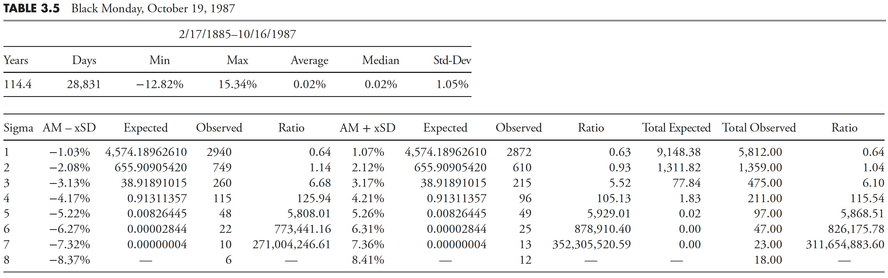
Black Monday, October 19, 1987
Desk 3.5 exhibits the boundaries for one to eight sigma across the arithmetic imply (AM) return for the interval from 2/17/1985 till the day earlier than Black Monday, October 19, 1987. Black Monday’s decline was 22.61 p.c, which is lower than the two-day decline in October 1929. Nonetheless, it was twice as massive as Black Tuesday, October 29, 1929, which is the day acknowledged by most historians because the day of the crash.
 Desk 3.5
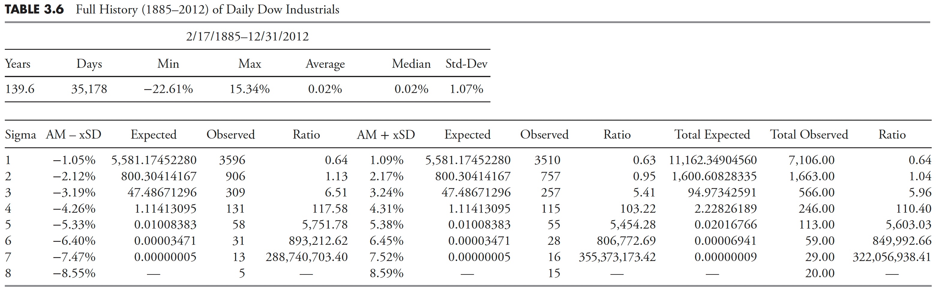
1885–2012
Desk 3.6 exhibits the boundaries for one to eight sigma across the arithmetic imply (AM) return for the interval from 2/17/1885 till 12/31/2012.
 Desk 3.6
Rolling Returns and Gaussian Statistics
This part makes an attempt to point out that top sigma is a way more frequent occasion than fashionable finance thinks it’s. Quite a few examples utilizing the Dow Industrials again to 1885 every day are proven. Every begins with setting a look-back interval to find out the typical day by day return and the usual deviation, after which a look-forward interval is ready to see if the look-back information continues into the look-forward information.
Determine 3.2 is an try to assist visualize this course of. A glance-back interval is decided (in-sample information) and a look-forward interval can be decided (out-of-sample information). The look-back interval is used to find out the typical day by day return and the usual deviation of returns. From that information, a variety of three sigma in regards to the imply is decided. Then within the look-forward information, the variety of day by day returns exterior the +/- 3 sigma band are tallied, with the entire being displaying as a plot; any level on the plot represents the information used within the look-back and the look-forward intervals.
 Determine 3.2
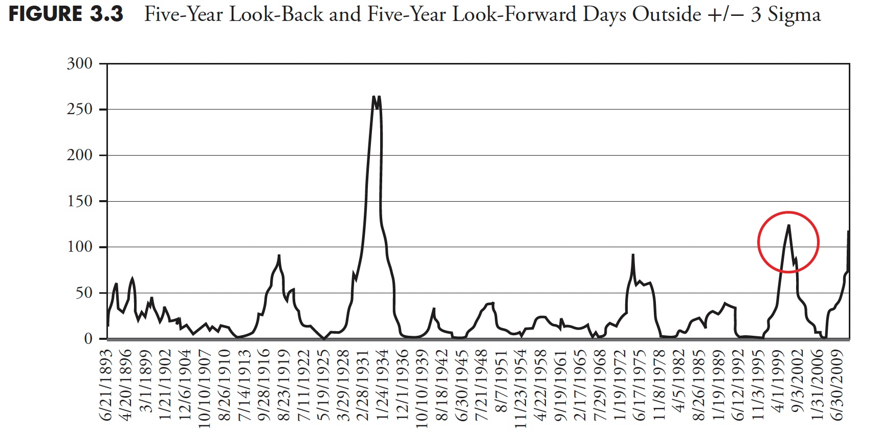
In Determine 3.3, a look-back interval of 1,260 days (5 years) is used to calculate a median day by day return and the usual deviation of returns. On 10/24/2002 (circle on Determine 3.3) the typical return over the previous 1,260 days was 0.07 p.c, and the usual deviation over the identical interval was 0.71 p.c. Subsequently, a 3-sigma transfer up was as much as 2.21 p.c, and a 3-sigma transfer down was -2.06 p.c. The look-forward interval, additionally 1,260 days, is counting the variety of days during which the returns have been exterior of the look-back vary. There have been 49 days with returns larger than 2.21 p.c and 69 days with returns lower than -2.06 p.c, for a complete variety of days with returns exterior the +/- 3 sigma vary (primarily based on the earlier 5 years) equal to 118. Desk 3.7 places this into one other format.
 Determine 3.3
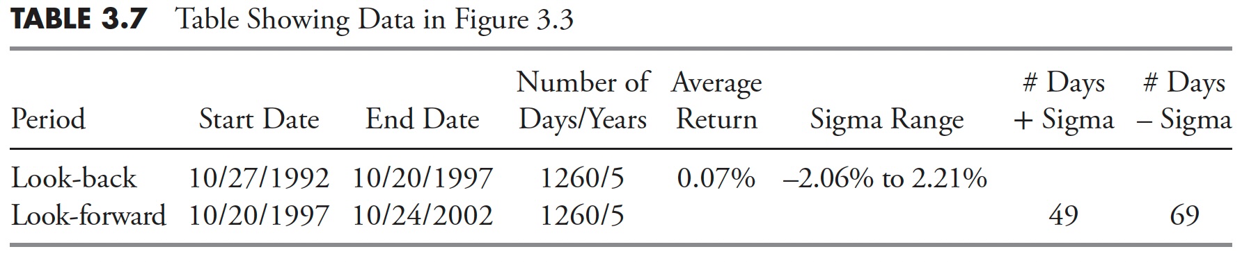 Desk 3.7
For a +/- 3 sigma occasion, the anticipated variety of observations must be 1.7, whereas there have been 118, which is 59 occasions greater than anticipated (occasions have to be in complete numbers, so we’re utilizing 2 for the anticipated quantity). Determine 3.3 exhibits the 1,260-day rolling whole variety of days exterior the +/- 3 sigma vary. As of 12/31/2007, the entire is 116, with an expectation of only one.7. That is greater than 58 occasions extra returns exterior the +/- 3 sigma band than anticipated. Of these 116 days exterior the 3-sigma band, 54 have been above 2.45% and 62 have been under -2.37%.
Lowering the look-forward interval to 1 yr (252 days) whereas sustaining the five-year look-back interval yields the chart in Determine 3.4 of rolling variety of days exterior a +/- 3-sigma (normal deviation) occasion. Keep in mind that the dedication of +/- 3 sigma is decided by the earlier 5 years of knowledge at any level on the chart. For a one-year look-forward, there may be solely an expectation of 0.34 occasions (days) exterior the sigma band.
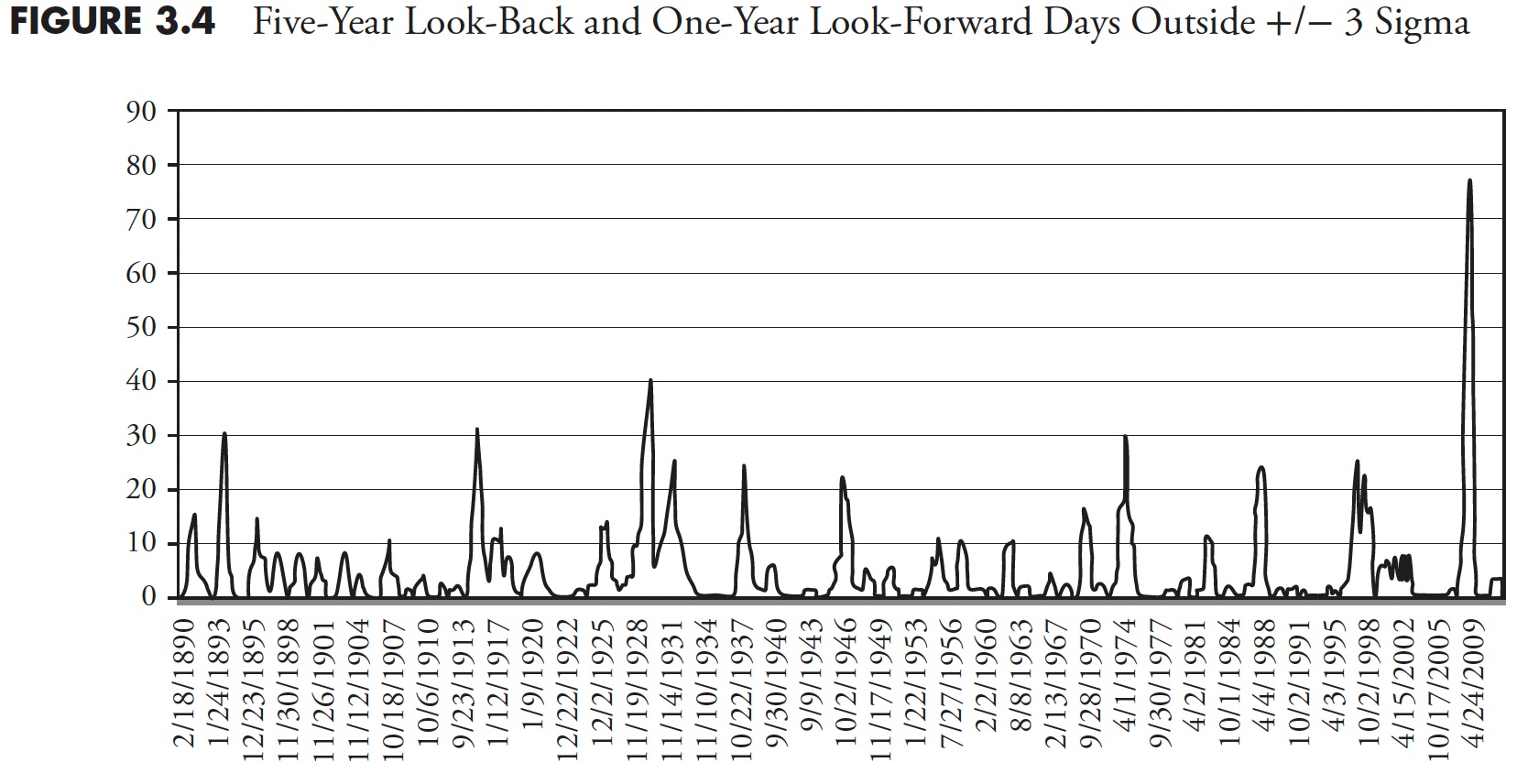 Determine 3.4
Taking this idea to a different view, Determine 3.5 exhibits the rolling variety of days exterior the +/- 3 sigma band for a look-forward of 1 yr and a look-back of 10 years (2,520 days).
Conserving the look-forward interval to 1 yr and increasing the look-back interval to twenty years (5,020 days) is proven in Determine 3.6. This chart is sort of much like the earlier one, with solely a 10-year look-back. Extrapolating the previous into the longer term at all times has its surprises. Conserving the look-forward interval the identical (one yr) and rising the look-back interval doesn’t considerably have an effect on the rolling returns exterior the sigma vary.
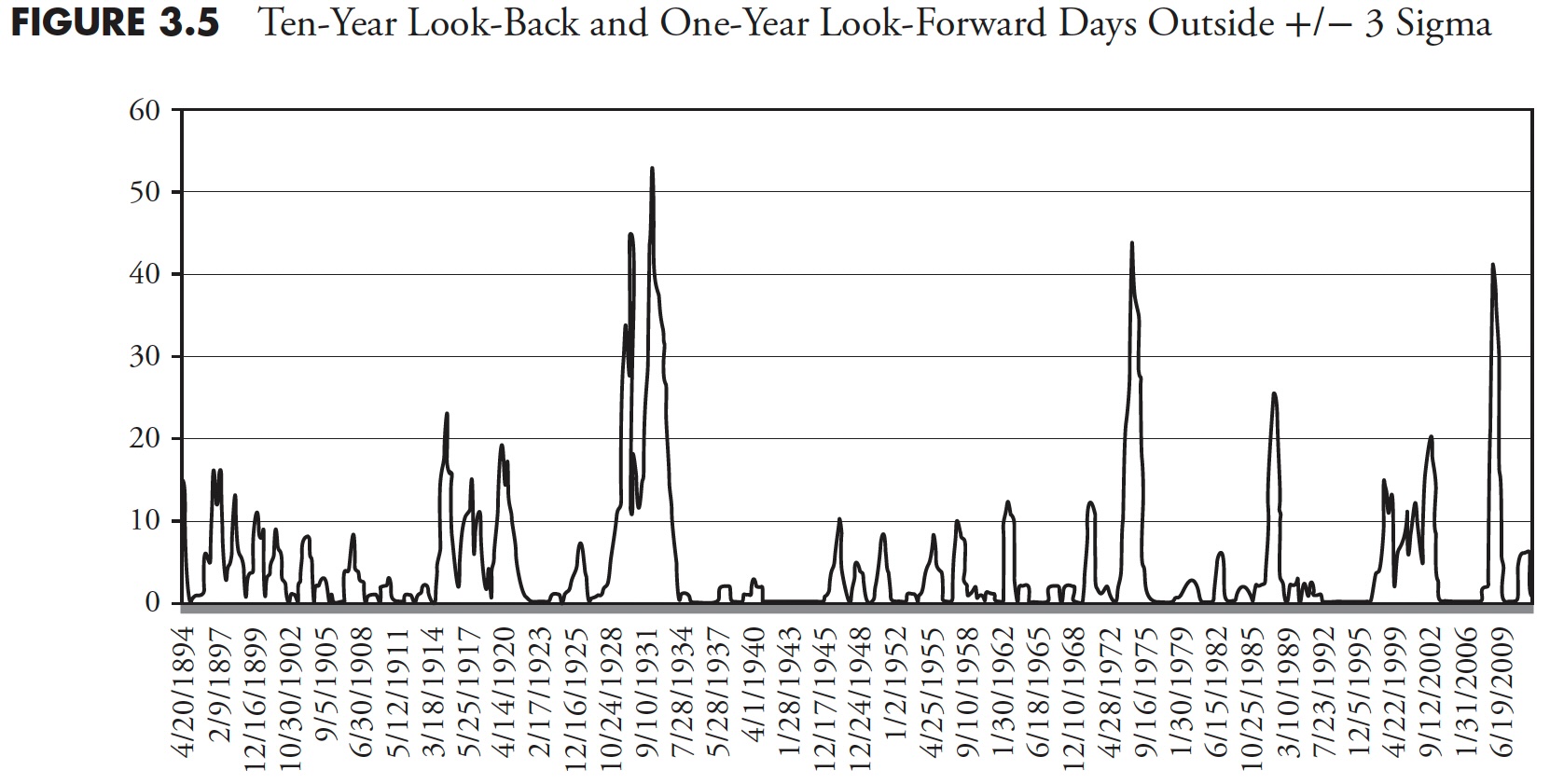 Determine 3.5
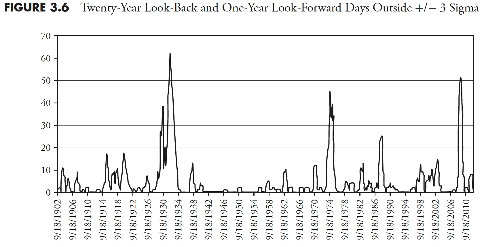 Determine 3.6
Lastly, in Determine 3.7, taking a 50-year look-back interval (12,600 days), as anticipated, the variety of occasions the next yr had exceeded the +/- 3 sigma envelope was related.
Backside line: Gaussian (bell-curve) statistics will not be acceptable for market evaluation, but fashionable finance is completely wrapped up in utilizing normal deviation as volatility after which saying that’s danger. There are literally two massive issues: one is using normal deviation to signify danger, and two is that previous normal deviation has little or no to do with future normal deviation. The primary downside doesn’t account for the truth that normal deviation (sigma) can be measuring each upside strikes and draw back strikes with no try and separate the 2. Clearly, upside volatility is nice for long-only methods. The second downside was adequately coated on this part exhibiting how insufficient normal deviation is from the previous in predicting how it could be sooner or later.
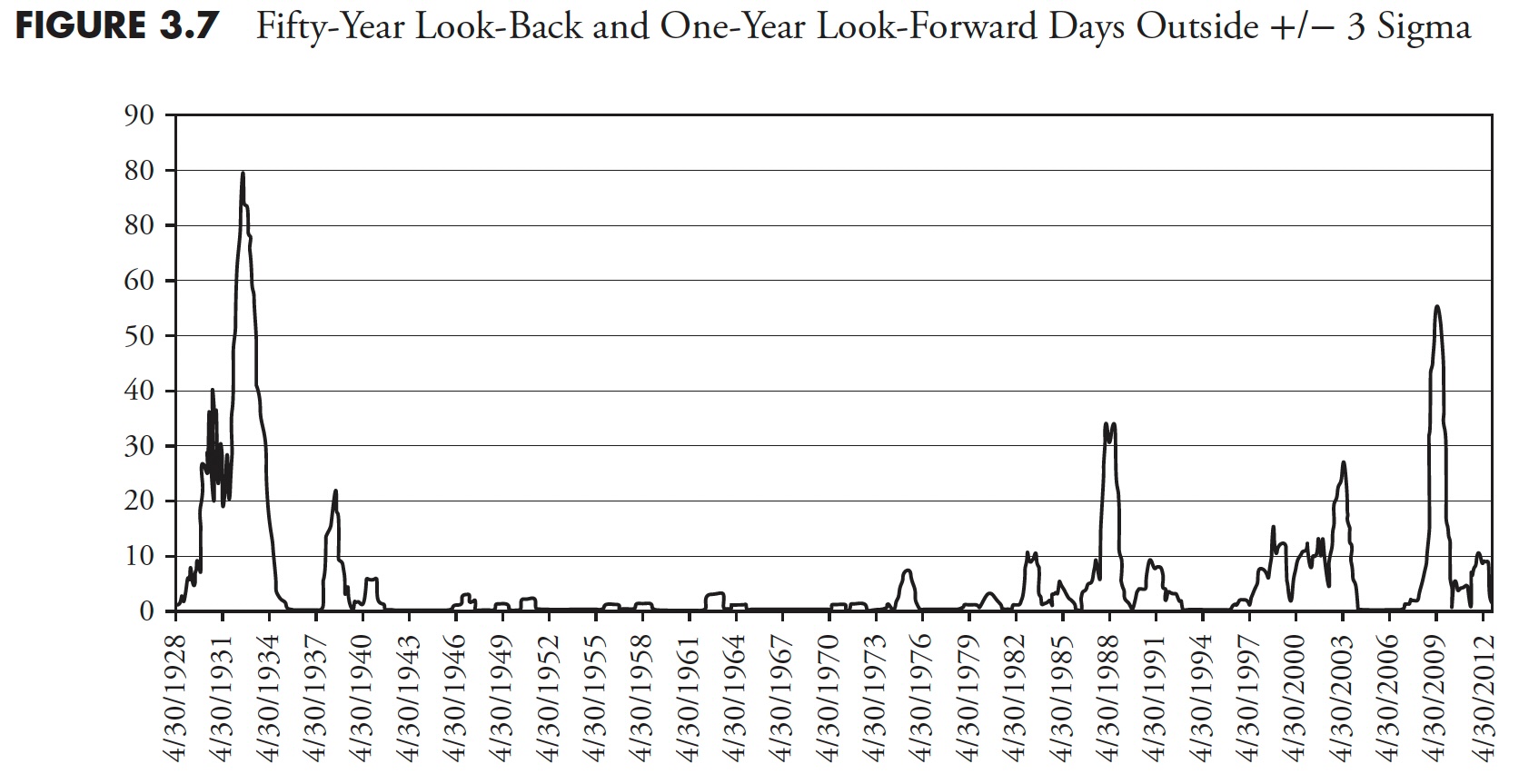 Determine 3.7
Thanks for studying this far. I intend to publish one article on this collection each week. Cannot wait? The e book is on the market right here.